There exists various articles online that discuss Bayer based image dithering, but I was not able to find one that simultaneously discussed how the threshold matrices used in the technique were constructed and provided source code with a working example. Consequently, I wrote this short article for anyone seeking such a quick reference.

Overview

Image dithering is a method that can be applied to reduce colour banding present in low bit depth (pallet limited) images, and was a common post processing step when it was not possible to print images using a sufficient number of colours (either due to mechanical limitations or cost) to avoid artifacts.

Next to noise (random) dithering, with simply randomly sample the image and apply a fixed threshold to each pixel value, ordered dithering methods are the next simplest to implement and use. Principle among these is Bayer dither, which is the technique discussed and implemented below.

Ordered (Bayer) Dithering

Bayer dithering, and ordered dithering in general, make use of a matrix of threshold values that are compared to each pixel value in the image to quantize colours. More specifically, for a \(n\)-by-\(n\) matrix \(T\), the, \({\rm RBG}\), colour channel values of each pixel, \({\rm pixel}(x,y)\), are quantized to \(c\) values based on the rule:

Bayer threshold matrices are a special class of matrices, constructed by (Bayer, 1973) for the task of create an “optimal distribution”, which can be taken to mean “pleasant to the eye”, of dots within the resulting image. The most commonly used matrices are those constructed using the following recursive block matrix formula, as seen on Wiki,

with the initial matrix value

which has entry values ranging from \(0,1,\dots,2^{2n}-1\).

Implementing Bayer Dithering

Bayer based image dithering is straightforward to implement for three channel images following the above description of the method. A working example implemented using JavaScript and the p5.js graphics library.

let c     = null; //number of grey levels
let d     = null; //dimension of threshold map
let M     = null; //threshold map
let img   = null; //image reference
let img_Y = null; //bitmap array of relative luminance values of img
let img_D = null; //final dithered image

function preload() {
  //initilize constants
  c = 4;
  d = 8;
  //define threshold map
  M = [[0,32,8,40,2,34,10,42],
       [48,16,56,24,50,18,58,26],
       [12,44,4,36,14,46,6,38],
       [60,28,52,20,62,30,54,22],
       [3,35,11,43,1,33,9,41],
       [51,19,59,27,49,17,57,25],
       [15,47,7,39,13,45,5,37],
       [63,31,55,23,61,29,53,21]];
  for(let i=0; i<d; i++){
    for(let j=0; j<d; j++){
      M[i][j] = M[i][j]/(d*d); 
    }
  }
  //load image and allocate space for luminance image
  img   = loadImage("assests/mike.jpg");
  img_Y = new Array(img.width*img.height);
}

function setup() {
  //no loop canvas
  noLoop();
  pixelDensity(1);
  createCanvas(img.width,img.height);
}

function draw(){
  img_D = createImage(img.width,img.height);
  img_D.loadPixels();
  img.loadPixels();
  for(let i=0; i<img.height; i++){
    for(let j=0; j<img.width; j++){
      let idx = 4*(i*img.width+j);
      let T = M[j%d][i%d];
      img_D.pixels[idx  ] = 255*Math.floor(T+img.pixels[idx]*(c-1)/255)/(c-1);
      img_D.pixels[idx+1] = 255*Math.floor(T+img.pixels[idx+1]*(c-1)/255)/(c-1);
      img_D.pixels[idx+2] = 255*Math.floor(T+img.pixels[idx+2]*(c-1)/255)/(c-1);
      img_D.pixels[idx+3] = 255;
      }  
  }
  img_D.updatePixels();
  image(img_D,0,0);
}

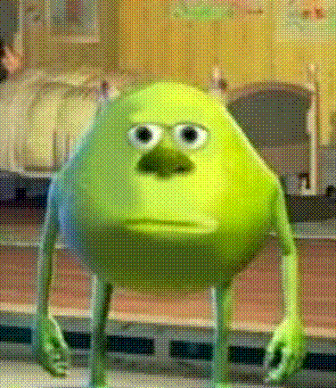
The above method performs decently well on a variety of different subjects. As an example, take the Bayer dithered image of Mike Wazowski with parameter values \(c=4\) and \(d=8\).

Take as another example, the dithered picture of a hotel I saw whilst in Honolulu for ICML2023.